All published articles of this journal are available on ScienceDirect.

Analysis of Eco-efficiency and its determinants among Smallholder Vegetable Producers in Eastern Ethiopia
Abstract
Introduction:
This study aimed to analyse eco-efficiency and its determinants for small holder vegetable producers in Eastern Ethiopia. Multi-stage sampling was used to select 256 small-scale vegetable producers in the study area.
Methods:
The study employed Data Envelopment Analysis to estimate eco-efficiency and Tobit model to identify the sources of differences in the eco-efficiency of farmers. The results of the DEA model revealed that the mean of eco-efficiency was 0.75, indicating that there is still a chance of improving the environmental performance of the farms without compromising the economic output of the farms.
Results:
The results of Tobit depicted that age, education, training, and adoption of sustainable intensification practices positively affect eco-efficiency, while farm size, farm income, and leadership status of the farmer negatively influence the eco-efficiency of the farm.
Conclusion:
Due emphasis should be given to promoting the adoption of SIPs and introducing an inclusive approach to educating farmers in the study area.
1. INTRODUCTION
Agriculture is still the dominant sector in the development of the Ethiopian economy. Agriculture in Ethiopia has been considered a source of food, income, and employment. However, the sector is still characterized by low productivity, small-scale and subsistence farming [1], environmental degradation, and adverse climate change. Transformation of the sector is mainly linked to the continuous expansion of land and labour productivity through policy-induced intensification [2]. Hence, most of the time, the growth in agricultural production including vegetables was at the expense of environmental costs like deforestation, reduction in biodiversity [3, 4], water pollution, land degradation, soil erosion [5, 6], and unfavourable climate change (Xiang et al.,2020). Farmers’ excessive usage of chemicals, fertilizers, and pesticides with the intention of sustaining certain levels of productivity has been seriously damaging soil structure, soil fertility [7], human health, and other ecosystems.
Failure of smallholder farmers to sustain farm productivity, the unsympathetic impact of agricultural activities on the environment, the lack of conservation, and the inefficient utilization of natural resources, opened a new room for researchers to introduce the concept of eco-efficiency in agriculture. Furthermore, Ethiopia is listed among low-income and food-deficit countries, meeting the current and future demand for food for its swiftly increasing population in a sustainable manner without imposing a burden on the environment, further elucidating the importance of measuring the eco-efficiency of agricultural production.
The term “eco-efficiency” has emerged in the past decades as a practical tool to measure sustainability [8]. It is an analytical method that evaluates the efficiency of economic processes not only from a traditional input perspective that ignores production-related externalities but also considers their accompanying burdens on the surrounding environment and land resources [9].
At the micro level, eco-efficiency means selecting the appropriate technology or production practice that has the least environmental impact, as well as a selection of raw materials and resources that reduce their consumption and enable the provision of high-quality products [10]. Initially, the concept of eco-efficiency has been applied by manufacturing companies in the 19th century to evaluate the impact of economic activities and decisions on the environment (Lehni, 2000). Gradually, as the impact of agriculture on the environment became larger, the necessity to diminish the environmental burden on the one hand [11], and the ever-increasing world demand for food on the other [12] initiated the concept of eco-efficiency to be introduced in agriculture to accentuate the optimum utilization of natural resources and minimum emission of wastes and pollution.
In Ethiopia, land constraint is a challenge where 87% of farmers possess less than two hectares of cropping land [13, 14]. The undergoing of environmental degradation through the exploitation of land, forest, and water resources could have an impact on the deteriorating agricultural productivity of smallholder farmers and exacerbate environmental problems in the country.According to the knowledge of the researcher, there is no single study that assessed eco-efficiency and its importance in tackling both low agricultural productivity and environmental problems concurrently at the farm level in Ethiopia. In light of this context, this study will be intended and performed to answer the following vital research questions:
1. What are the levels of smallholder vegetable producers’ eco-efficiencies?
2. What factors determine smallholder vegetable producers’ eco-efficiency?
The objectives of this study were:
1) To measure the eco-efficiency of smallholder vegetable producers;
2) To identify factors that affect the eco-efficiency of smallholder vegetable producers.
Hence, this study is considered a stepping stone that encourages farmers to engage in a type of environmental-friendly production that will neutralize or minimize detrimental usage of natural resources and commercial agricultural inputs to the least possible amount, while sustaining or even enhancing the level of production.
2. CONCEPT OF ECO-EFFICIENCY
Different type of terminology referring to eco-efficiency has been developed, but until now there is no commonly agreed definition of eco-efficiency [15]. According to Huppes [15], eco-efficiency is the ratio of value created per one unit of environmental impact. World Business Council for Sustainable Development defines eco-efficiency as: “creating more goods and services with less use of resources, waste, and pollution” [16].
Eco-efficiency is considered a double-edged instrument that can assess issues pertaining to economic and environmental aspects concurrently. Hence the reason why, Schaltegger et al. [17] stated that the prefix “eco” refers to both “economics” and “ecology”. From an economic perspective, the focus is on maximizing the desirable output from a given amount of input or using the minimum possible quantity of inputs without compromising the predetermined amount of output. While from an ecological aspect, the intention is to minimize the consumption of environmental resources (substituting with environment-friendly inputs) in a sustainable manner so as to minimise undesirable outputs like wastes, emissions, and pollutants that are detrimental to the environment.
Eco-efficiency measures the relationship between economic growth and environmental pressure and is generally expressed by the ratio between economic value and environmental influence, represented by the following equation:
Eco-efficiency=Production Value/Environmental Impact [18]. In the agricultural context, measurements of eco-efficiency are expressed in one of the following ways: 1) eco-efficiency is explained as more desired output/less undesired output. For example, reducing over-fertilization, such as N-fertilizer use on cereals in China [19], or over-irrigation such as with irrigation volumes on sugarcane in north-west Australia [20].
2) Eco-efficiency is described as equal to a lot more to a little more. For example, production levels were increased through careful targeting of production inputs such as “micro-dosing” maize or sorghum with N fertilizer in southern Africa [21]. 3), Eco-efficiency is equal to more with the smarter use of the same. For example, raising the effectiveness of current agricultural inputs through better targeting these inputs in space, such as via precision agriculture [22], or time, for example, with a seasonal climate forecast [23]. 4), Eco-efficiency is explained as less to much less. For instance, minimizing production in areas where inputs are not efficiently used (e.g., for climatic or soil reasons) and shifting resources to areas of better eco-efficiency [24].
3. MATERIALS AND METHODS
3.1. Description of the Study Area
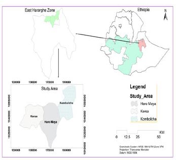
The study was conducted in the East Hararghe zone of the Oromia Regional State of Ethiopia. It has a total population of more than 35.1 million [25]. East Hararghe Zone (Oromo: Godina Harargee, Bahaa) is one of the Zones of the Oromia Regional State of Ethiopia. East Hararghe Zone is bordered on the Southwest by Bale, on the West by West Hararghe Zone, on the North by Dire Dawa, and on the North and East by the Somali Region. The Zone is geographically located between 7°32′-9°44′ North latitude and 41°10′-43°16′ East longitude with an altitude ranging from 500 to 3405 meters above sea level [26]. East Hararghe Zone is well known for vegetable production. According to Central Statistical Agency [25], the total area allocated for vegetable cultivation in East Hararghe was estimated as 544.30 ha which generated nearly about 33,175.33 quintals of vegetables. The zone has 18 administrative districts (Fig. 1).
3.2. Sampling Technique and Sample Size
Following previous studies [27, 28], a multi-stage sampling technique was used to select the sample units. The first stage involved purposive sampling where three districts were purposively selected from 18 districts of the East Hararghe Zone by considering their high potentiality in vegetable cultivation capacity. Following the purposive sampling of the districts, the second stage involved stratified random sampling to stratify the list of kebeles into vegetable producers and non-vegetable producers. Then, by using a simple random sampling method, three vegetable producer kebeles were selected from each district (i.e., a total of nine kebeles) proportional to size. An equal number of kebeles was drawn from each district due to the similarity (in number) of the kebeles making up a more considerable amount of vegetable-producing kebeles in each district. Given the population size of the study area, the total sample size was determined using a formula that provides the maximum size to ensure the desired precision using the formula given by Kothari [29] as follows:
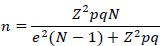 |
Where n is the desired sample size; Z is the standard cumulative distribution that corresponds to the level of confidence with the value of 1.96; e is the desired level of precision; p is the estimated proportion of an attribute present in the population with the value of 0.5 as suggested by Israel [30] to get the desired minimum sample size of households at 95% confidence level and ±5% precision; q=1-p; and N is the size of the total population from which the sample is drawn. Accordingly, a sample of 256 farm household heads was selected from nine kebeles using random sampling with probability proportional to size.
3.3. Data Types, Sources, and Methods of Data Collection
In this study, both primary and secondary data were used. Secondary data was gathered from several sources including the East Hararghe Zone agricultural office, woreda agricultural and rural development offices of the three woredas, reports, and documents of sampled kebeles and non-government organizations. Face-to-face personal interviews using a semistructured questionnaire were employed to collect primary data. Both open and close-ended types of questions were included in the questionnaire to collect information relevant to the purpose of the study. The questionnaire was pretested before conducting the field survey to crosscheck the understanding status of enumerators to the questionnaire and for appropriateness (format, content, clarity, adequacy, and sequence of questions), and review based on the feedback from pretesting.
3.4. Methods of Data Analysis
This study included both descriptive statistics and econometric analysis to estimate the values of the unknown parameters of the population and testing of hypotheses. Descriptive statistics such as means, standard deviation, ratios, proportions, frequencies, etc. were used to capture the multidimensional behaviour of the households and farms in the study area. Data envelopment analysis (DEA) and two-limit Tobit models were employed for measuring eco-efficiency and its determinant eco-inefficiency, respectively.
As noted earlier, this study prefers measuring the eco-efficiency of targeted farms using the DEA approach as it involves only a limited number of a priori assumptions concerning the functional relationship between inputs and output [31]. In DEA, the production frontier is constructed as a piecewise linear envelopment of the observed data points. It does not require not only identical units of measurement for the different inputs and outputs but also familiarity with their relative prices.
In this regard, the Decision-Making Units (DMUs) encircled by the envelope are considered inefficient. Following either the input or output-oriented model of DEA, DMUs should adjust their inputs or outputs to move to the frontier. In the input-oriented DEA, the frontier minimizes inputs for a given level of output, while in output-oriented DEA the frontier denotes the maximum output which could be attained using a given input level.
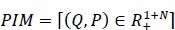
As mentioned earlier, we have defined eco-efficiency as the ratio between economic value added and environmental pressure. Following Picazo-Tadeo [32], let us now assume that we observe the economic value added or desirable output, denoted by Q, generated in the production processes by a set of f = 1,…, F farms. Besides, the production process generates a set of t =1,….. T damaging environmental pressures also appeared at the farm level, which is represented by P = (p1,……. Pt). The Production Intensification Method (PIM) consists of various activities that generate desirable output (Q) and environmental pressure p is defined as:
 |
(1) |
Desirable output Q could result in generating environmental pressure P. Hence, the formal definition of eco-efficiency of farm f (EEf) is written as:
 |
(2) |
“P” refers to the pressure function that aggregates the “t” environmental pressures into a single environmental pressure score. The desirable output Qf on the numerator of the Eco-efficiency ratio can be calculated depending on the direct primary data collected on the prices and quantity of output. Formally expressed as:
 |
(3) |
However, with issues pertaining to computing the denominator, it is worth noticing that constructing the composite environmental pressure score is a common challenge for researchers in measuring eco-efficiency as the different aspects of an environmental pressure composite indicator need the adoption of a weighting scheme to assign relative importance to each pressure [33]. Although, Ripoll-Bosch [34] generated a weighting scheme on a farm regarding intensification depending on the workshops conducted at the farm level [35], argued that the use of a subjective weighting scheme can result in conflict and biased weights. That is why Kortelainen [36] proposed that a rational way toward calculating this score is to take a weighted average of the specific pressures undertaken by farm f on the environment. This technique allows weights to be determined at the farm level. It is formally computed as:
 |
(4) |
Where Wnf is the weight with which n pressure enters into the computation of the composite environmental pressure indicator for f farm. In this study, the pressure function that aggregates the environmental pressures is specified as follows:
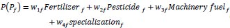 |
(5) |
Then, through DEA, eco-efficiency scores for each farm belonging to the benchmarking sample of f = 1,……. F farm were calculated from the following fractional programme. Eco-efficiency for the fth farm is maximised subject to the constraint that all efficiency measures must be less than or equal to one. Therefore, the mathematical formulation of the relative eco-efficiency of the DMU can be found by using the following model proposed by Charnes et al. [31]:
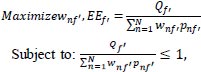 |
(6) |

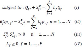
It is mostly the easiest way for decision-makers to focus merely on the eco-efficient DMUs. Nevertheless, decision-makers often encounter the challenge of how to undertake additional comparisons among the eco-efficient DMUs. Thus, the following duality form of model (6) also offers information about the minimization of environmental pressure or an increase in desirable outputs for the DMUs to move from eco-inefficiency to eco-efficiency.
 |
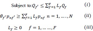 |
(7) |
Lf indicates a set of intensity variables representing the weighting of each detected farm f in the composition of the eco-efficient frontier. Lf is also considered the standard for a particular farm. The reference set will provide coefficients for the Lf to framework the theoretically efficient farm. The efficient target exposes how environmental pressures can be minimized to make the farm more eco-efficient and maintain a balance between environmental pressure and economic value added. θf denotes the eco-efficiency score for each of the f farms. The estimate will satisfy the restriction θf, ≤1 with the value θf,=1 referring to an eco-efficient farm.
The critical point that needs to be raised here is that the eco-efficiency score that will be gauged by applying equation (7) is not based on Pareto-Koopmans efficiency but rather on [31] efficiency measures that depend on the weakly efficient frontier. This approach merely investigates the possible amount of the farm’s environmental damage required to be minimized radially for a farm to attain eco-efficiency. Such kind of efficiency is known as weak DEA efficiency [37], which implies that even if DMU has score efficiencyθ*f=1, still there is room for minimizing the environmental burden or improving the desirable output without compromising the economic value added or opting for other additional inputs. Such an optimal solution reveals the presence, if any, of a surplus in inputs and a shortage in output called slacks. As a result, Charnes et al. [31] introduced the additive model of DEA that directly deals with input surplus and output shortage. Furthermore, within the framework of DEA,Ali A et al. [38] and Picazo-Tadeo et al. [32] explained, the slack can be calculated from the optimising programs as follows:
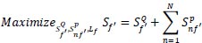 |
 |
(8) |
SP and SQ indicate pressure slacks (excesses) and value-added slack (shortfall), respectively. According to Picazo-Tadeo et al. [32], the objective of description (8) is to maximise the sum of pressure excess and value-added shortfalls at a farm level while maintaining their ratio of eco-efficiency scores at the level computed from the expression (7). Accordingly, if there is positive slack, we can say that the farm is Farrell efficient even if additional reduction of inputs or improvement of output is feasible to some extent. Thus, expression (8) has the power of evaluating the eco-inefficiency of a farm by a slack-based efficiency score after environmental pressures are adjusted to their minimum level. Besides, Sherman et al [37]. used excess in the use of inputs identified by slacks to identify and assess the sources of economic inefficiency. In this manner, any excess in environmental pressure indicates the presence of an intensified production method that could minimize or abstain from exerting excess pressure on the environment without affecting output. This creates an opportunity for farmers to further improve their productivity while simultaneously focusing on the reduction of excess in the use of environmentally damaging inputs [33].
Torgersen et al. [39] estimated the potential environmental pressure reductions in the intensified production methods towards the improvement of the economic and environmental efficiency of the farm. Following Torgersen et al. [39], the aggregate reduction of n pressure required to bring farm f into a Pareto – Koopmans efficient status is computed by adding together radial reduction and pressure-specific excess. Formally:
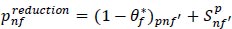 |
(9) |
Sp is representing pressure slacks (excesses). The first term on the right-hand side of formula (19) gauges the proportional reduction of pressure n, while the second term computes the slack in the direction of these environmental damages. Similarly, the Pareto-Koopmans efficient level of pressure n is computed as follows:
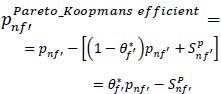 |
(10) |
Finally, the pressure-specific measure of eco-efficiency for farm f' and pressure n is figured as the ratio between the Eco-efficient level of that damage and its actually observed level in order to account for the total proportional reduction in that pressure needed to bring farm f' into a Pareto – Koopmans efficient status.
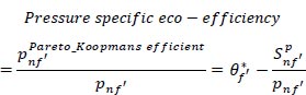 |
(11) |
The importance of slacks in explaining pressure-specific Eco-efficiency can be evaluated by measuring the weighting of potential pressure reduction due to slacks based on the total pressure potential reduction. The above relationship can be expressed formally for pressure n as:
 |
(12) |
 being the pressure n that would result from the radial contraction of all environmental pressures of farm f towards its eco-efficient reference on the frontier.
3.5. Determinants of Eco-efficiency
To deal with the determinants of eco-inefficiency of farm households in vegetable production, several environmental, socio-economic, and institutional variables were regressed on eco-inefficiency estimates using a two-limit Tobit regression model. The Tobit model was deployed because the efficiency scores are double truncated at 0 and 1 as the scores lie within the range of 0 to 1. The tobit model that uses the maximum likelihood becomes a better choice to estimate regression coefficients [40]. The functional form of the two-limit Tobit model is:
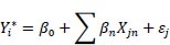 |
(13) |
Where Y*i = latent variable representing the efficiency scores of farm j, β = a vector of unknown parameters, Xjn = a vector of explanatory variables n (n = 1, 2, ..., k) for farm j and Ɛj = an error term that is independently and normally distributed with mean zero and variance σ2.
Representing Yi as the observed variables, we have:
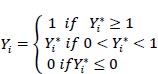 |
(14) |
In this expression, the distribution of the outcome variable is not normally distributed, rather its value varies between 0 and 1, if the data to be analysed contain values of the dependent variable that is truncated or censored. Hence, the OLS is no longer applicable to the concept of estimated regression coefficients. The overall fitness of the two-limit Tobit model will be checked based on the chi-square test statistic displayed on top of the model outputs. In addition to the overall fitness, diagnostic tests on multi-collinearity of the explanatory variables, heteroskedasticity test, and model specification errors will be made using VIF (Breusch-Pagan/Cook-Weisberg test) and RAMSEY RESET tests, respectively.
4. RESULTS AND DISCUSSION
4.1. Analysis of Farm Eco-efficiency using the DEA Method
This section presents and discusses the results of farm eco-efficiencies estimated using the DEA method. As it was explained in chapter three, DEA used economic value added (desirable output) and environmental pressure, i.e., gross profit margin as economic value added and cost of fertilizer, chemical, fuel, and farm specialization ratio as indicators of environmental pressure, to undertake both economic and environmental improvement evaluation of smallholder farmers at farm level.
From the collected sample respondents, farmers that did not apply or use one of the above variables were omitted as it is impossible to compare with the other farmers that applied all of them. Besides this, it is highly recommended to fulfil the requirements and features of the data set that the DEA requires to enable the model straightforwardly executed. For instance, fulfilling the positivity requirement of the DEA model must be because DEA cannot generate a complete analysis with negative and zero numbers. Another requirement that DEA data should fulfil like some authors [41] mentioned is keeping the magnitude of the data set quite similar since the imbalance of the magnitude of the data set may cause a round-off error problem. To ensure this fulfilment, we preferred expressing the amount of fuel purchased by the farmer in a jar (20L) instead of litres and the economic value added (desirable output) in quintals. Accordingly, a total of 256 farms that fulfilled the requirements of the DEA data set were selected to undertake the analysis of eco-efficiency. A summary of both economic variables and environmental pressure is stated in Table 1 below.
Before running the model, the following pre-processing analysis of some statistical characteristics of the data sets was implemented. To begin with, the normality of the data was tested using Z-score and box plot method and thereby verified the normality of the data. One thing we have to be aware of regarding DEA is that it is highly sensitive to outliers as it accounts for all deviations from the frontiers due to inefficiency. Hence, to assure the robustness of the efficiency results of DEA to outliers of both desirable output and environmental pressures, to deal with outliers in the data, the method applied by Ripoll-Bosch et al. [34] was employed. Finally, R package version 4.2 was used to estimate eco-efficiency with the farm understudy.
In Table 2 below, the results of DEA indicated that the mean score of radial eco-efficiency for the overall sample was 0.75. The majority of the farm, nearly around 60% of the farms had efficiency scores greater than 0.7, 16% had efficiency scores greater than 0.9, and only less than 2% of the farms had efficiency scores less than 0.5. A total of 16 farms had scored 1 eco-efficiency, i.e., on frontiers, and constituted only 7% of the sample. This denotes that generally, the eco-efficiency of the farmers was better although there is still a great room for the farmers to maximize the environmental improvement while maintaining the economic value added. In a nutshell, the results obtained from the mean radial score of eco-efficiency may set guidance to the sample farmers that they can on average minimize the currently exerted environmental pressure on their farm by 25%.
| Variable | Unit | Mean | Std. Dev. | Min. | Max. |
|---|---|---|---|---|---|
| Environmental pressure | |||||
| Inorganic fertilizer | qt/ha | 2.331 | .976 | 1 | 6 |
| Pesticide | Kg/h | 2.108 | .773 | 1 | 4 |
| Fuel | Jar/ha | 12.039 | 1.788 | 6 | 16 |
| Farm specialization ratio | # | .603 | .274 | .1 | 1.2 |
| Economic variable | |||||
| Desirable output | qt/ha | 59.906 | 6.22 | 45 | 77 |
| Range of Eco-efficiency | Freq. | Percent | Cum. |
|---|---|---|---|
| 0.1< = E < 0.5 | 6 | 2.34 | 2.34 |
| 0.51< = E < 0.6 | 27 | 10.55 | 12.89 |
| 0.61< = E < 0.7 | 67 | 26.17 | 39.06 |
| 0.71< = E < 0.8 | 79 | 30.86 | 69.92 |
| 0.81< = E < 0.9 | 39 | 15.23 | 85.16 |
| 0.91< = E < 0.99 | 16 | 7.42 | 92.58 |
| E = 1 | 16 | 7.42 | 100.00 |
| Total | 256 | 100.00 | - |
| Variable | Obs. | Mean | Std. Dev. | Min | Max |
|---|---|---|---|---|---|
| Inorganic fertilizer | 256 | .71 | .207 | .25 | 1 |
| Pesticide | 256 | .655 | .237 | .25 | 1 |
| Fuel | 256 | .847 | .145 | .5 | 1 |
| Farm specialization ratio | 256 | .503 | .234 | .1 | 1 |
It is critical to note that radial eco-efficiency is essential in assessing the maximum proportional reduction of environmental pressures that farmers can attain. However, being radial eco-efficiency is known as weak eco-efficiency, it is impossible to address the specific pressure to be reduced in a specific direction. These potential reductions of specific pressure in a specific direction are only attainable by Pareto - Koopmans eco-efficiency. As a result, there is a small variation between the two scores, i.e., radial eco-efficiency and Pareto-Koopmans eco-efficiency, and clearly, the Pareto-Koopmans eco-efficiency score is less than radial. As it can be seen in Table 3 below, on average pressure, the specific eco-efficiency score of inorganic fertilizer, chemical, fuel, and farm specialization ratio is 0.71, 0.65, 0.84, and 0.50 respectively.
The importance of estimating pressure-specific eco-efficiency will be clearly elaborated by interpreting the results of pressure-specific eco-efficiency along with the radial eco-efficiency of a given farm. To begin with, let us pick farm number 154 from the sample and inorganic fertilizer for pressure-specific estimation. As indicated in Appendix II, this farm had a radial eco-efficiency score of 0.84, which denotes that the farm has the possibility of reducing environmental pressure by 16% without affecting the economic benefit to be generated from the farm. In other words, to visualize the integration of the concept of eco-efficiency with that of sustainable intensification, the amount of fertilizer that the owner of the farm applied to the farm in the past production period which was 1.5 kg was beyond the environmental carrying capacity of the farm. Specifically, the farmer exerted an extra 16% (0.24 qt) of fertilizer that deteriorate the soil structure and affect the future productivity of the farm in a sustainable manner.
Aside from this, the Pareto-Koopmans score of pressure-specific eco-efficiency of inorganic fertilizer was estimated as 0.78, which connotes that the farm has still the potential of reducing specific environmental pressure (inorganic fertilizer) by 22% (0.33qt) while achieving the predefined economic target. Generally, the sum of the radial eco-inefficiency score (0.24qt) and pressure-specific eco-inefficiency score (0.33qt) gives us the total possible amount of inorganic fertilizer that the owner of this farm should reduce to minimize the environmental burden along with producing the maximum attainable level of production.
Concerning the issue of proper utilization of environmentally detrimental inputs, the farmers in the study area had mentioned, during FGD, that the majority of them have still a skill gap pertaining to the optimum level of input to be applied. Those who had skills and enough understanding were raised that they are not implementing their skills because it is a time-consuming and tedious task. Hence, they prefer applying those inputs arbitrarily without paying any attention not only to the risk of depletion of environmental resources and the associated costs but also without taking into consideration the problem of high agricultural commercial input constraints the country is currently encountering. As a result, the eco-efficient farmer may reap at least three benefits viz. solving the problem of commercial input scarcity, ensuring the conservation of ecosystems that in turn can serve the farmer from various perspectives, and generate sustainable desirable output from the farm.
The last critical point of great importance to be raised regarding DEA results is the information one can obtain from the assigned optimal weights of DEA and reference units. In the case of interpreting the eco-efficiency of a given farm from the weight point of view, the optimal DEA weight assigned points out the percentage of attention that the farmers can pay for each or a given specific pressure to improve environmental performance potential. For example, farm number 9 assigned 45% weight for inorganic fertilizers, 32% weight for pesticides, 15% weight for fuel, and 8% weight for farm specialization ratio. This entails that the owner of the farm gave higher emphasis to inorganic fertilizers than the others to boost environmental performance.
In the same manner, reference units have also an eye-catching implication, such that DMU should use the assigned reference units as a benchmark. This is because DEA could not offer the appropriate practices (solutions) through which a given DMU (in our case farm) can solve the problem of eco-inefficiency rather DEA directs eco-inefficient DMUs to reference units from which eco-inefficient units can get proper guidance and advise that enable the eco-inefficient unit to operate at the frontier.
4.2. Results of Determinants of Eco-efficiency
After estimating eco-efficiency, identifying the factors that determine eco-efficiency is inevitable to offer the full package of research on the topic as it enables farmers, practitioners, researchers, policymakers, and all other stakeholders to easily obtain concerned information from the study as an input to get their output as per their goal. Determinants of eco-efficiency were estimated using the Tobit model.
Table 4.
| Eco-efficiency | Coeff. | St.Err. | t-value | p-value | ||
|---|---|---|---|---|---|---|
| Sex | -.002 | .02 | -0.09 | .929 | ||
| Age | .003 | .002 | 1.92 | .056* | ||
| Fsize | -.005 | .003 | -1.80 | .073* | ||
| Education | .021 | .002 | 8.38 | 0.00*** | ||
| Experience | -.001 | .002 | -0.69 | .488 | ||
| Irrigation | -.013 | .021 | -0.65 | .518 | ||
| Leadership | -.027 | .016 | -1.72 | .087* | ||
| Extensions | .004 | .027 | 0.14 | .891 | ||
| Media | .037 | .025 | 1.47 | .143 | ||
| Farmslope | -.005 | .004 | -1.26 | .209 | ||
| Livestock | .004 | .004 | 1.19 | .234 | ||
| Amount | -.001 | 0 | -3.86 | 0.00*** | ||
| Training | .036 | .014 | 2.57 | .011** | ||
| Tillage | .012 | .014 | 0.83 | .408 | ||
| Rotation | .035 | .016 | 2.21 | .028** | ||
| Organicfertilize | .054 | .016 | 3.39 | .001*** | ||
| Constant | .575 | .057 | 10.09 | 0.00*** | ||
| var(e | .011 | .001 | .b | .b | ||
| Mean dependent var | 0.754 | |||||
| Pseudo r-squared | -0.378 | |||||
| Chi-square | 116.697 | |||||
| Akaike crit. (AIC) | -389.463 | |||||
Source: own computation from the survey (2022).
A model diagnostic test was conducted to check the acceptability of the results of the model. A multicollinearity test was conducted and the results disclosed that the mean VIF was 1.5 and the maximum VIF was 3.5. This expresses that there is no Multicollinearity in the data set (Appendix 4). Breusch-Pagan / Cook-Weisberg test was also made to test the problem of heteroskedasticity and the result of the test proved that there is no problem of heteroskedasticity in the model. Breusch-Pagan / Cook-Weisberg test for heteroskedasticity (Ho: Constant variance Variables: fitted values of eco-efficiency chi2 (1) = 0.14, Prob > chi2 = 0.7131). Model specification test (Ramsey RESET test) was made, and the result publicized that there is no problem with model specification in the model (Ramsey RESET test using powers of the fitted values of eco-efficiency, Ho: model has no omitted variables, F (3, 238) = 0.31, Prob > F = 0.8173).
Before presenting and discussing the results obtained from the model, it is worth noticing that, in chapter three we mentioned that demographic, socio-economic, institutional variables, and farm features were hypothesized to influence eco-efficiency in the study area. The results of the Tobit model in Table 4 portrayed that eco-efficiency was significantly influenced by age, household size, education, leadership, income from the farm, and adoption of sustainable agricultural intensification practices.
The age of the household positively and significantly affected eco-efficiency. The possible explanation is that older farmers are predicted to have better awareness of farming and technical skills accumulated through their lifetime. This drives the older farmers toward increasing the eco-efficiency score of their farms. For marginal effect analysis, the coefficient of age revealed that as the age of the household increases by one year, the probability and level of farm eco-efficiency increase by 0.3 percent. Similar to our results, Gadanakis et al. [33] found a positive impact of age on the eco-efficiency of the farm. However, Resti A and Godoy-Durán et al. [42, 43] found a negative coefficient of the age of the farmer indicating that young farmers were more eco-efficient than older farmers but their result was insignificant.
Household size had a negative influence on eco-efficiency at a ten percent level of significance. Farmer with high numbers of family members was found more eco-inefficient than farmer with fewer family members. A one-unit increase in household size decreases the likelihood of eco-efficiency by 0.5 percent. Initially, it was anticipated that a family member is a source of labour that enhances both productivity and environmental performance concurrently, which in turn affects eco-efficiency positively. However, the result found was opposite to what was expected and hypothesized before. The possible justification behind the negative effect of household size on eco-efficiency was the issue of food security and covering the basic needs of the family. As the size of the family increases, the effort of the farmer on ensuring the family’s food security and providing the basic needs of life to the family increases. This encourages the farmer to exhaustly utilize the existing environmental resources which in turn negatively affects the eco-efficiency of the farm.
The results of the Tobit model showed that the education of the farmer in the study area has a positive and significant effect on the eco-efficiency of the farmer. Specifically, a unit increase in the year of schooling would increase the probability of eco-efficiency by 0.02 percent. The result found was congruence with that of Gadanakis et al. [33] who found a similar result i.e. the positive effect of education level on the score of eco-efficiency. This may be due to the fact that farmers with high education levels may be quite better not only in their managerial skills but also in estimating and applying the optimum levels of agricultural inputs on the farm. Another reason that supports the result is that educated farmers are superior in easily obtaining and processing useful information and making better decisions than illiterate farmers. Considering that few studies conducted on eco-efficiency found the effect of education on eco-efficiency insignificant. For instance, Kortelainen et al. [36], who studied the eco-efficiency of high-yielding variety rice in Bangladesh, found an insignificant effect of education factors on eco-efficiency.
This study also found the leadership status of sample respondents as one of the most influential factors that caused variation in the score of eco-efficiency among farmers in the study area. As it is demonstrated in Table 4, the leadership status of the farmer is negatively and significantly related to eco-efficiency. The plausible reason behind this issue is identical to the point mentioned by some of the participants in the focus group discussion that is, currently the farmer that holds any leadership position in the society, became busy with various duties and obligations to be discharged by the leader. A leader farmer has not enough time to engage in farm activities appropriately and on the other hand, holding leadership status gives them the chance to easily get access to commercial agricultural inputs in abundance. Hence, they use those inputs in surplus which in turn negatively affects the eco-efficiency of the farm.
Income from the farm had a significant and negative effect on the eco-efficiency of the farm. Besides, the computed marginal effect of farm income showed that one ETB increase in farm income would decrease the overall probability and level of eco-efficiency by about 0.1 percent. Reduction in eco-efficiency with the increase in farm income may be due to the fact that the farmers mostly did not give much attention to the amount of environmentally harmful agricultural inputs to be applied to the farm. This directly deteriorates the environmental performance of the farm. Moreover, the farm that generates higher income from the farm invests a tremendous amount of capital on irrigation and other similar activities and thereby exploits the environmental resources above the optimal ratio. This reason was supported by Zhong, F et al. [44] who found similar results to this study. Contrary to this result, Sabiha et al. [45] found a positive relationship between farm income and eco-efficiency but with no justification stated.
Farmers’ participation in training significantly influenced the level of farm eco-efficiency in the study area. It is apparent that training nourishes farmers with wide assets of knowledge, technical skills, and valuable information on how to enhance environmental sustainability and utilize agricultural inputs appropriately. Similar to this study, Heidenreich, A et al. [46] and Perez Urdailes et al. [47] found that access to training had a significant and positive effect on improving the eco-efficiency of the farm.
Adoption of sustainable agricultural intensification practices affects eco-efficiency significantly and positively, indicating that farmers that adopt SAIPs are more eco-efficient than that of non-adopters. This is because; those practices enhance soil improvement and preserve the existing environmental resources along with providing better economic yield. For instance, the estimated marginal effect of organic fertilizer showed that a unit increase of organic fertilizer would increase the probability of eco-efficiency by 5 percent. Weltin, M. et al. [48] also found that farmers’ adoption of sustainable intensification practices are highly associated with ecological improvement potential and an increase in eco-efficiency of the farm.
CONCLUSION AND RECOMMENDATION
The empirical investigation of the eco-efficiency of the farmer at the farm level was computed by the non-parametric DEA model. The overall average farm household’s eco-efficiency (EE) generated from the results of the DEA model was 0.75. The result further pointed out that the majority of the farm, nearly around 60% of the farm, had efficiency scores greater than 0.7, 16% had efficiency scores greater than 0.9, and only less than 2% of the farms had efficiency scores less than 0.5. To further advance the eco-efficiency scores of the farm and minimize the prevailing environmental pressure, examining the factors that influence the eco-efficiency of the farm is very crucial. This is because it helps policymakers design appropriate policies and set a mapping road for practitioners and other stakeholders. To this effect, the Tobit model was employed to identify factors that influence eco-efficiency scores within the farm in the study area. The results of the model illustrated that EE was positively and significantly influenced by age, education, training, and adoption of SAIPs. The results also revealed that family size, leadership status of the household head, and income from the farm had significant and negative effects on the eco-efficiency of the farm in the study area.
Overall, the results indicated that there is still good potential for improving the environmental performance of the farm without compromising the existing farm output. Hence, due attention should be given regarding the optimum utilization of environmentally detrimental commercial agricultural inputs. The result of eco-efficiency obtained from this study was limited to only a few agricultural inputs. Therefore, to further address the negative impacts of commercial agricultural inputs on the environment and natural resources, conducting wide and experimental-oriented research that can address the magnitude and extent of the effect of each input should be emphasized. Furthermore, inviting various private, governmental, non-governmental, and other concerned bodies to provide training and awareness to increase farmers’ access to training on optimum utilization of commercial agricultural inputs and conservation of environmental and natural resources should be given policy attention to maximize the eco-efficiency score of farms.
LIST OF ABBREVIATIONS
| EE | = Eco-efficiency |
| DMUs | = Decision-Making Units |
| DEA | = Data envelopment analysis |
ETHICAL STATEMENT
The study was approved by the institutional ethic committee of Haramaya University, Agricultural Economics.
CONSENT FOR PUBLICATION
Not applicable.
AVAILABILITY OF DATA AND MATERIAL
All the data and supporting information are provided within the article.
STANDARDS OF REPORTING
COREQ guidelines were followed in this study.
FUNDING
None.
CONFLICT OF INTEREST
The authors declared no conflict of interest financial or otherwise.
ACKNOWLEDGEMENTS
Declared none.