All published articles of this journal are available on ScienceDirect.

Applying Operation Research Methodologies to Hydroponic Crop Scheduling in a Closed System: An Integer Programming Approach
Abstract
Background:
Hydroponic system has spread across Europe, but its use in developing countries is limited. Hydroponics may represent the industrial version of farming. It is established within buildings; it depends on automation, can go vertically, and has better use of land resources. However, the feasibility of hydroponic farms is hindered by the start-up cost and may be improved through the proper scheduling of the harvest to be in the optimal duration to take advantage of price seasonality and traditional farming production fluctuations.
Methods:
To improve the feasibility of hydroponic farms, this work develops a new operation research model that includes sales price variations, volume and productivity of plants, space limitations, electrical installation, solar panels, etc. This model aims to address the most important questions that farmers face, that is, what, when and how much to plant. Certain assumptions are made, such as reusable packaging, solar panels, and limiting the plantation to selected popular crops in Jordan that can be easily marketed. The model is applied to a farm of size equal to 500 m2 in area and 4000 m3 in volume.
Results:
The main result of this work is the valuable figure that shows the plantation schedule. It shows the timely plantation (how much and when) for each type of the selected plants. Further analysis is performed regarding the profit and total plant volume as compared to the total volume of the farm. It also evaluates actual production versus target production.
Conclusion:
This work evaluates the expected profit of the selected hydroponic farm to be 17,778 JD compared to an average of 1000 JD from traditional farming of land with the same square meters.
1. INTRODUCTION
The feasibility of hydroponic systems in third-world countries is questionable due to competition with low-cost traditional farming. Traditional farming is characterized by relatively low start-up costs and production costs, as well as relatively low sales prices. However, the production and the sales price of traditional farming are characterized by fluctuation and seasonality. Seasonality production of traditional farming results in large quantities of the same crop sent to the market at relatively the same time, leading to lower sales prices. Traditional farming also suffers from the need to use an extensive amount of land and the need for a relatively large volume of water for irrigation. Conveniently locating traditional farms near cheap sources of water may distance them from consumers; thus, more transportation cost is incurred. High transportation cost forces farmers to harvest a large amount of crops to justify the transportation cost. The high amount of exhibited products in the market and the low shelf life of these products lead to lower sales prices. Hydroponic has an extensively lower need for irrigation water and thus may be conveniently located near the consumers. The lower transportation cost may reduce the need to harvest except what the consumers order, thus taking advantage of the higher sale price.
On the other hand, a hydroponics system suffers from higher costs of energy, installation, and nutrients while having the advantage of the closeness to customers, level production across the years, lower need for water than traditional farming, the ability for vertical build-up (use of 3D space), and the successful integration of solar panels. Hydroponics has lower viability if established in the same spots as traditional farming, if they harvest in the same seasons as traditional farming, or if they do not include solar panels or other energy-saving systems to reduce energy costs.
Closed-type (indoor) urban agriculture may be the most viable form for hydroponics in third-world countries. Urban areas comprise half of the world's population and are expected to rise to more than 70% by 2050 [1]. The rise of the population in urban areas makes it more important to promote urban agriculture (UA), which is efficient in terms of water and nutrients [2]. Urban agriculture (UA) has the advantage over traditional farming due to the reduction of long-distance transportation costs [3, 4]. UA can also have the advantage of using city wastes and the advantage of improved energy efficiency by using buildings and rooftops [5-7]. Moreover, UA can use solar panels to supply the plants with the necessary lighting for their growth, which can affect the economics and the feasibility of the farms. In urban areas, more cities want to develop sustainable and local food systems by integrating local UA. UA can assume a diversity of forms, such as community gardens, allotments, guerrilla gardening, rooftop gardens, greenhouses, and aquaponics [8]. In this context, commercial micro-farms are raising interest because their small scale seems particularly convenient in urban areas with restricted access to land [9].
Crop planning is concerned with the selection of crops and the assignment of land area (both land location and land size) for maximizing profit while including several factors, such as economic, biological, physical, social, weather, markets, and costs through the use of budgeting or/and mathematical programming [10]. In modern industries like farms, scheduling can be used as a synonym for planning, as this is the more common name in the industry. Planning is usually associated with quantifying the amount of resources needed to fulfill the anticipated demand, while scheduling allocates the planned resources to the production in a timely manner to deliver the ordered products to the customer at the proper time without delay. In that respect, allocating areas to crops is similar to allocating machines to products. While planning can be used to quantify the total area needed, the total number of machines needed, etc., in an aggregate manner.
Spatial land decisions were the subject of many research works, which included single and multi-objective optimization and other techniques [11-13]. Land use management in the context of crop planning has also been the subject of extensive early research, for example, in the context of spatial distribution and resource allocation [14-20]. The same crop planning problem may be formulated as goal programming. Goal programming is a special multi-objective formulation that may include profit, water limitations, market limitations, etc., which, in turn, are summed up to one figure after multiplying each separate objective by a suitable weight to reflect its importance [21]. The crop planning problem may also be formulated to include the crop succession requirements to determine the best sequence [22]. Crop rotation may also be included in the formulation [23]. Crop planning or scheduling may be formulated and solved to include sustainability and profitability to maximize production volume or revenues by determining the best division of various heterogeneous pieces of land under known demands [24]. Moreover, it can be used to schedule the best planting dates and harvest dates for specific plants [25]. Some crop planning formulations seek maximal profit while having a limited amount of water and crop seeds [26, 27]. It may also consider the existing groundwater irrigation system [28]. Other studies attempted to minimize the total irrigation water and maximize the net income from farming and the total agricultural output [29]. The crop planning formulation may also determine the crop rotation (specific crop patterns in consecutive planning periods) by maximizing the profit and considering hard constraints for environmental impact with no limitations of irrigation water [30]. Other formulations attempt to optimize both crop-planning and zoning through the integration of the Delineation of Rectangular Management Zones (DRMZ) with the Crop Planning Problem (CPP) in precision agriculture. The first problem consists of partitioning the agricultural fields into chemical and physical management zones satisfying a specific homogeneity level considering the soil properties. These partitions are commonly used to improve agricultural practices, such as fertilization, irrigation, pest control, etc. The second problem considers the management zones to determine the best crop for each plot maximizing the profit [31]. Other models attempted the minimization of waste generated by the use of resources necessary for the task of crop maintenance in a similar manner to Lean Manufacturing (LM), which includes labor, use of machinery, and operations in time windows that preserve the quality of harvest [32].
Operations research or/and optimization have been used within hydroponic context, to alter the cultivation factors to optimize the biomass production [33], alter ammonium/nitrate and potassium in nutrient solution to optimize bulb fresh weight, bulb dry weight, and whole-plant dry weight [34], alter component ratio (hydroponic tank volume to rearing tank volume) to optimize fish growth, vegetable yield, and nutrient removal [35], retrofit a light industrial building with a hybrid renewable energy-assisted hydroponics farming to optimize crop production [36], alter commonly known hydroponic parameters, such as hours of illumination, photosynthetic flux density, temperature of nutrients, concentration of nutrients, etc., to optimize plant growth [37], the modification of spectral distribution and light intensity (i.e., light intensity, duration, and spectral distribution) for maximum cost effectiveness and reducing carbon footprint [38], alter the anion composition of the nutrient solution by using an experimental design with the independent variables, NO3-, H2PO4-, SO4-2 and Cl-, to optimize two response variables: number of leaves and forcing efficiency [39], apply reinforcement learning, artificial intelligence, and Internet of Things (IoT) to optimize the amount of water for irrigation [40], alter stocking density to optimize length and weight gain, nitro blue tetrazolium (NBT) activity and catalase activity, glucose, and cortisol level in aquaponics system [41], and to use different fertigation management practices to explore the impacts of agronomic performance and environmental life cycle [2].
Farm crop planning is affected by fluctuations in prices, which represent a tangible risk for farms' feasibility [42, 43]. Crop prices are affected by farm production and farm inputs [44]. The environment has a definite influence on the quality and quantity of the harvest in traditional farming. Open non-controlled farms may also suffer from weeds, pests, etc., which may lead to more risk for the harvest [45-50]. In this respect, closed indoor urban farms are more immune to these risks and may lead to more stable production and a reliable supply chain. However, these farms use more technology and have high start-up investment costs. Also, closed hydroponic farms have less need for water, which is nearly 3% of what is used for traditional farming. Also, closed indoor hydroponic farms may be implemented vertically, and this is extremely important as it has higher production per square meter. They also have less risk for weeds, pests, etc. problems. Properly designed hydroponic farms are usually automated and are characterized as lower labor intensive than traditional farming. However, some tasks that cannot be automated will still be done manually. Automation and control can be used for monitoring, irrigation, nutrient addition, concentration control, and weather management tasks. Increased automation, powered irrigation, and the lighting system will require more energy; therefore, installing a suitable PV system will reduce the energy cost significantly. This is especially true for countries like Jordan, which gets excessive sunlight.
In this work, we consider the optimization of vertical farms by adding a new concept, namely the 3d or volume perspective. Mostly, if not all, previous research work was devoted to allocating areas. This work may have the novelty of allocating volume to plants, not surface areas. This work attempts to optimize the crop scheduling or crop planning problem in 3D, which is more suitable for vertical farming. This work also includes the variability of volume and price all year round. It takes into consideration the different costs, including labor, seeds, installation, etc., in one number. An increase in the volume consumed by the plant with time due to growth is also considered. The model assumes energy cost to be included in the initial investment through installing a sufficient PV system. This research work shows the variation in the prices for different types of crops over the year and suggests an optimization model for the profitability of the hydroponic system. The decision variable is important to farmers, that is: “what to plant and how much to plant year-round” to achieve the highest profit. The model assumes that the selected farm is in an urban area with trivial transportation costs. It also assumes that the system is already built with enough solar panels to exclude energy costs. Depreciation costs for the built system and maintenance costs are also included.
2. METHODOLOGY
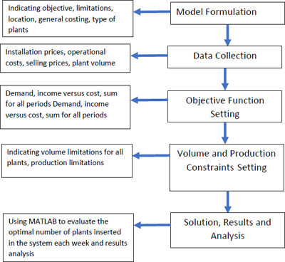
Fig. (1) shows the methodology devised for this work. It starts with a model formulation which includes limitations, setting objectives, general costing, and the type of plants included in this work. The next step is data collection, which explores the installation price, operational costs, and possible selling prices for the produce and the volume taken by each type of plant on a weekly basis. Model construction includes two main steps, which are objective function setting and constraints settings, which are then used to develop the operations research model. The model is then solved in MATLAB to answer the most important questions in relation to farming, which is what and when to plant to attain feasible and profitable production. The results are further analyzed and validated.
2.1. Volume Allocation
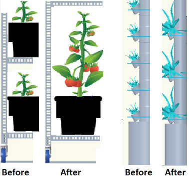
Mechanical engineering design can be used to develop flexibility in the shape of the plant containers. Fig. (2) shows some methodologies, such as flexible shelves design, where the size and the height of the shelve can be modified to accommodate more plants when they are small by using lower shelves when plants are just planted and germinated while the shelves can be moved up to accommodate plants when they have grown. Also, Fig. (2) shows another popular hydroponics system in pipes, where extension pipe units can be added as the plant grows to accommodate the larger size of the plant.
Fig. (2) illustrates the allocated volume of the plant, which is an imaginary cuboid drawn around the plant. The plant volume allocated should be modified to include its portion of the service lane. The volume of the plant should include its own volume in addition to the volume of the service, such as lighting, irrigation, and service lanes.
3. MODEL DEVELOPMENT
In farming, the objective will be to maximize profit. This maximization will ensure the viability and continuity of the project. The most important decision variable for the farmers is what to plant and how much of each type. Due to seasonality, the choices are limited for traditional farming. However, considering indoor farming with controlled conditions, seasons are not there. There are fewer or even no season limitations. Therefore, the decision variable will be what to plant and when. Producing in and out of season when the prices are high can be the economic edge, where hydroponic systems can flourish and prosper. This is extremely important considering the huge price variability for the different products. The price may double across the year. It is difficult for traditional farming to take advantage of these price fluctuations, but hydroponics can.
Considering the optimization of the decision variable, in this model, we selected a typical urban farm to choose the number of plants to be planted in the system. Weeks were selected as the variable decision point for both cultivation and plantation. Thus, they can be defined as:
XTi:Number of Tomato/ new tomato plants placed in the system in Week i
VTij: Volume occupied by tomato plant placed in the system in week i, in week
PTij: Production in Kg of tomato plant placed in the system i in week j
STij: Sales prices of tomato plant produce for plant placed in the system in week i, in week j
CTij: Cost weekly of tomato plant produce for plant placed in the system in week i, in week
DTj: Anticipated demand for tomato plants produce in kg in week j
The same can be considered for other plants: (
Let us define:
Xij = [ XT ;XCa;XS;XO;XL;XP;XCu;XST;XCh;XG]
Vij = [ VT ;VCa;VS;VO;VL;VP;VCu;VST;VCh;VG]
Pij = [ PT ;PCa;PS;PO;PL;PP;PCu;PST;PCh;PG]
Sij = [ ST ;SCa;SS;SO;SL;SP;SCu;SST;SCh;SG]
Cij = [ CT ;CCa;CS;CO;CL;CP;CCu;CST;CCh;CG]
The profitability per plant is defined as:
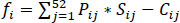
The model, in this case, can be stated as:

Subject to


4. MODEL CONSTRUCTION AND DATA COLLEC-TION
4.1. Objective Function
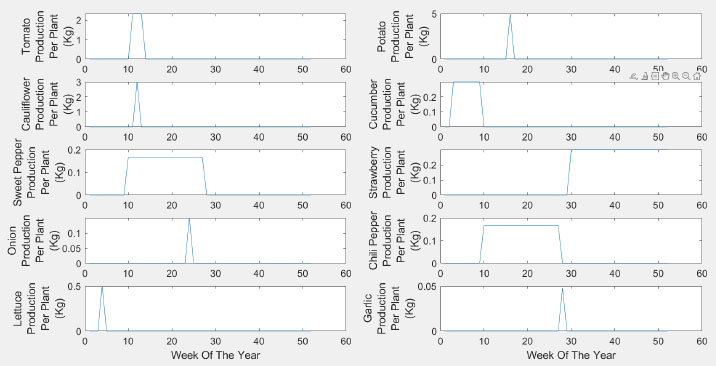
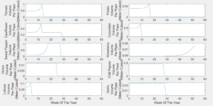
The income of hydroponics for the current model comes from the sales of vegetables. The farm under consideration is an urban farm within a city, and thus we can exclude multiple aspects that are usual costs for traditional farming, including major transportation costs, lost production due to insects or pests, wasted plants prior to sale, disposable packaging, supply chain costs due to direct sales to customers, etc. The assumption of zero or minimal waste is due to minimum handling and minimum transportation. The production per plant was obtained from previous studies [47-49] for all of the plants under consideration and is shown in Fig. (3). The objective function includes three variables, sales, production per plant, and cost. This kind of information is obtained from experts in the field and the Jordanian department of statistics [50]. For example, the tomato plant can produce in the 11th week after plantation, and it provides an average of 2.33 Kg each week for three weeks in a row. Fig. (3) illustrates this for the 10 plants of interest. Some plants have continued production for many weeks, such as chili pepper, while others produce once, such as garlic, onions, lettuce, and cauliflower. Fig. (3) illustrates that the plantation in the system is made in week zero if, in any case, the placement in the system is done in week i the whole curve is shifted to the right with weeks. For example, if a tomato plant is placed in the system in week 3, it will start to produce in week 14 (11 weeks from the zero-week plantation plus 3, which is the start of the plantation).
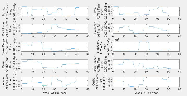
To obtain weekly pricing, we used certain officially selected references [51, 52]. Fig. (4) shows the seasonality for the different plants' prices at different weeks of the year. It is not unusual for the prices to double or even triple over a year. The prices are the lowest during high seasonal production. The highest pricing is noticed for out-of-season or in case of an event that resulted in damage to the traditional farming crops, especially due to uncontrolled weather conditions, such as very high or very low temperatures.
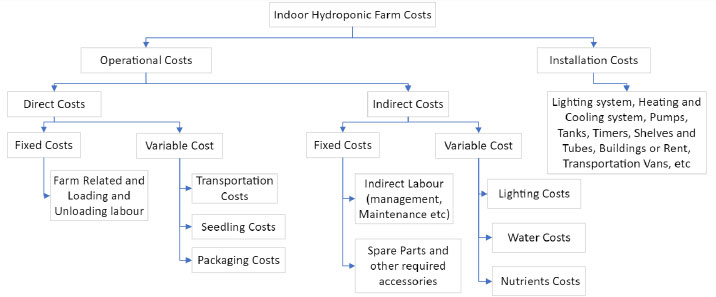
The last element for the objective function is the costing. Fig. (5) shows an illustration of some of the major costs incurred in hydroponics. The start-up or installation costs are the initial cost to start the whole farm. This cost includes the building, prototyping, rental, solar panels, control, A.C. systems, lighting and their maintenance, insulation, pumping systems, etc. The data for these fixed costs were collected with the help of experts to be nearly 180,000 JD. The project is assumed to live for 25 years, 52 weeks per year. The weekly cost is equal to 138.4 JD/ week. This cost is allocated to the different plants based on their volume percentage relative to the total volume.
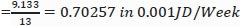
For this work, we have selected a hypothetical 4000 m3 (25 m × 20 m × 8 m) hydroponic farm assumed to run for 52 weeks, that is, 52 *4000 cubic meters * week. Although this is the total volume that can be used, including service lanes, the actually used volume based on our analysis is the sum of the total volume used, which is later evaluated in the paper to be 1.1245 *105 cubic meters*week. A tomato plant uses 7.2409 cubic meters*week, nearly an average of 0.5570 cubic meters for 13 weeks, including service lanes. It can be calculated as:


The other costs were allocated to the plants, including labor, in the same manner. The nutrition cost was major. The consumption per plant and the cost of these nutrients were obtained from agriculture experts.
The objective function, in this case, is just the multiplication of the production by the selling price minus the incurred costs (Equation 1). It can be observed that the profitability of the plants is variable because of the variability of the sales price. The cost is assumed to have a fixed value while the selling price is variable, and thus it is better to produce at weeks or periods when the market offers higher prices.
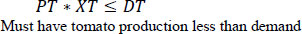
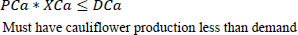
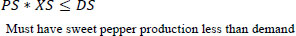
4.2. Volume and Production Constraints
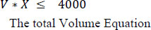
Constraints are shown in equations 2-16. Equation 2 is related to volume. Traditional outdoor farming is limited by the land size that is measured by square meters. Things are different in a properly designed hydroponic system; we can go vertically. The land is not the major issue; instead, we are limited by the volume. As discussed earlier, we evaluated the volume taken by the different plantations and placed that in the matrix (V). Vij is the volume taken by plant i in week j. Xi is the number of plants I placed in the system. XiVij is the weekly used volume for the 52 weeks; this value should be less than 4000 m3 (For this work, we have focused on constructing a 4000 m3 (25 m × 20 m × 8 m) hydroponic farm). Fig. (6) shows the volume consumed per plant starting from the day it is placed in the system.
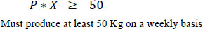
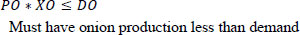
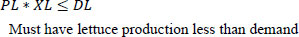
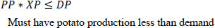
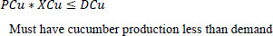
Equations 3 and 4 are related to production. Matrix P shows the weekly production of the plant in week J. X*P, in this case, represents the weekly production, which is assumed to be greater than a designated value of 50 Kg/week and less than the 2000 Kg/week. The 50 Kg ensures that there are sales and money in the system. However, 2000 Kg is the maximum that the farm should produce.
Table 1 shows the required maximum production for each type of plant based on local marketing assumptions. This may vary from farm to farm. Therefore, these numbers are specific for this considered hypothetical farm. Different farms will have different target values.
| - | Demand (kg) |
|---|---|
| Tomato | 479 |
| Cauliflower | 147 |
| Sweet Pepper | 200 |
| Lettuce | 100 |
| Potato | 432 |
| Cucumber | 315 |
| Onion | 257 |
| Strawberry | 200 |
| Chilli | 70 |
| Garlic | 50 |
| Sum | 2250 |
The actual weekly target varies according to the price. The demand is assumed to shrink at higher prices according to the following equation:

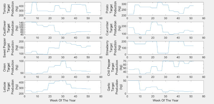
Fig. (7) shows the finalized target production.
5. MIXED INTEGER SOLUTION
Table 2 shows the Wallace [13] algorithm solution for the mixed integer problem. A full illustration of the solution is not included in this work. Instead, the solution to the problem is obtained through the MATLAB function, which may use the Wallace algorithm as a reference.
The MATLAB function to be used is intlinprog (f,A,b). This is suitable for integer programming problems subject to constraints.
[X,FVAL,EXITFLAG,OUTPUT] = intlinprog(f,A,b) which corresponds to
min f'*x over x
subject to: A*x <= b
x(i) integer, where i is in the index
The code for this function initiates the f, A, and b functions according to the model developed previously.
6. RESULTS AND DISCUSSION
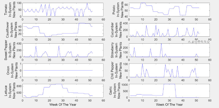
The MATLAB code is run to find the optimal 17,778 JD yearly profit. This is achieved based on selecting the solution of the decision variable X, as shown in Fig. (8). As can be seen in the figure, the number of plants placed in the system varies from week to week. Adhering to these numbers might increase the viability of hydroponic farms in Jordan. As expected, the lettuce proved to have a good portion for the production, which to a maximum of nearly 900 plants weekly in some cases. Also, it shows that some plants may not compete in a hydroponic system in terms of feasibility, such as onions. These plants are not optimal for hydroponics in Jordan. Garlic should be planted in specific weeks only.
Fig. (9) shows the weekly volume used by the plants. Although the current farm has 4000 cubic meters of space for plants, not all of that volume should be used based on optimization results. Fig. (10) shows the total kg production on a weekly base. Although the farm can handle up to 2000 Kg per week, the maximum suggested volume by the model is 1630 Kg, and it goes to as low as 1275 Kg per week. This limitation is affected by both the market prices and target production. Relaxing the target constraints will result in more plantation and an increase in the volume used.
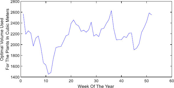
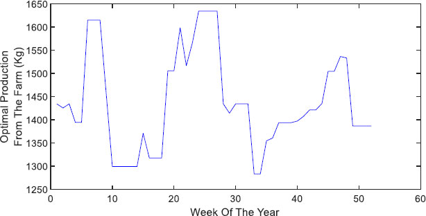
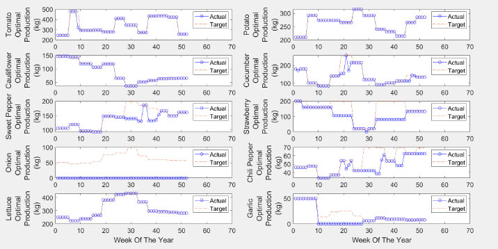
Fig. (11) shows the actual and target production for each plant. Most of the targets are met due to feasibility. Some plants are not suggested for plantation, such as onions. The same can be considered for sweet pepper, strawberry, chili, and garlic in some weeks.
CONCLUSION
This work is devoted to vertical hydroponic system optimization that includes sales price variations, the productivity of plants, and space limitations. The decision or input variable is how much, what, and when to plant. An operation research model was developed that included a profit objective function and constraints. The constraints included maximum volume and target production for each type of plant. The target production varies according to the price. It can be concluded that based on a square meter reference, the optimized hydroponic farms can be much more profitable than traditional farming. Adding the target production constraint may result in better sales but less utilization of the total possible volume. Some plants may not be profitable in hydroponic farming, such as onions, while others are profitable. The results of this work can be scaled down or up according to the size of the farms without much change in profitability per square meter, adding to the importance of the results of this work.
LIST OF ABBREVIATIONS
| UA | = Urban Agriculture |
| CPP | = Crop Planning Problem |
| DRMZ | = Delineation of Rectangular Management Zones |
| LM | = Lean Manufacturing |
ETHICS APPROVAL AND CONSENT TO PARTI-CIPATE
Not applicable.
HUMAN AND ANIMAL RIGHTS
Not applicable.
CONSENT FOR PUBLICATION
Not applicable.
AVAILABILITY OF DATA AND MATERIALS
The data and supportive information are available within the article.
FUNDING
This work was conducted during a funded sabbatical leave from The University of Jordan.
CONFLICT OF INTEREST
The authors declare no conflict of interest, financial or otherwise.
ACKNOWLEDGEMENTS
Declared none.